It’s so annoying trying to think of things to do. Sometimes you just want to type “epic night out” into Google Search and get what you’re looking for, right? I struggled with the same. So I built a semantic search app. It finds Foursquare venues in NYC leveraging Streamlit, Snowflake, OpenAI, and Foursquare’s free NYC venue data on the Snowflake Marketplace.

The semantic search lets users search for venues based on their intent (and not translating their intent to keywords). For example, users can search for venues for an "epic night out" or "lunch date spots" and find venues in their specified neighborhoods with Foursquare venue categories that are semantically closest to what they’re looking for.

In this first part of a two-part blog series, I’ll walk you through how I wrangled the data and implemented semantic search in Snowflake.

Why did I make this app?

I stumbled upon semantic search as I was exploring generative AI use cases. At its core, most semantic search apps use cosine similarity as a metric to determine which documents in a corpus are most similar to a user’s query. As I learned more about it, my inner Snowflake fanboy thought Snowflake’s impressive computational power and near-infinite scalability would be ideal for such a task! I wanted to power a semantic search app using Snowflake as an alternative to a vector database. Streamlit's Snowflake Summit Hackathon offered a perfect opportunity to do that.

Data wrangling

Step 1: Install the Foursquare NYC dataset from the Snowflake Marketplace

Before we get started, install the free Foursquare Places - New York City Sample from the Snowflake Marketplace (if you don’t have access to Snowflake, you can sign up for a 30-day free trial here). I shortened the default database to foursquare_nyc during installation.

After you install it, the data set will appear in the Snowflake UI:

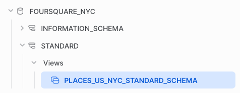
Foursquare provides a single view containing basic information about venues in NYC. We aim to leverage Snowflake to perform a semantic search of Foursquare venue categories. To achieve this, the columns we’re particularly interested in are fsq_category_labels and fsq_category_ids. fsq_category_labels contains an array of arrays. The outer array represents the list of categories. The inner array describes the hierarchy of the category, where the first element represents the root category and the last element represents the leaf category. fsq_category_ids contains an array of IDs for the leaf categories in the fsq_category_labels column.

Step 2: Set up a new database and schema

We’ll create a new database and schema to house our wrangled data:

-- Set up a new database and schema where we are going to house auxiliary data 
CREATE DATABASE foursquare;
-- Create a new schema
CREATE SCHEMA main;

Step 3: Create borough and (borough, neighborhood) relationships

From a user experience perspective, it’d be inefficient to comb through all NYC neighborhoods in each of the five boroughs. Also, querying a list of venues in a list of neighborhoods from the Foursquare dataset would be computationally expensive, given that the neighborhoods are stored as a string array in the neighborhood column. So we’ll create normalized tables to store information about NYC boroughs, neighborhoods, and which neighborhoods are in which boroughs.

First, we’ll create and populate a borough_lookup table:

CREATE TRANSIENT TABLE borough_lookup (
id number autoincrement,
name varchar
);

INSERT INTO borough_lookup(name) values
('Brooklyn'),
('Bronx'),
('Manhattan'),
('Queens'),
('Staten Island');

Next, we’ll create and populate a neighborhood_lookup table:

CREATE TRANSIENT TABLE neighborhood_lookup (
id number autoincrement,
name varchar
);

INSERT INTO neighborhood_lookup(name)
SELECT DISTINCT n.value::string
FROM foursquare_nyc.standard.places_us_nyc_standard_schema s,
table(flatten(s.neighborhood)) n
ORDER BY 1;

Next, we’ll create a borough_neighborhood table to store our (borough, neighborhood) mapping by:

• Creating a temporary table to store the manually curated (borough, neighborhood) mapping (find the exact insert statement here):

CREATE OR REPLACE TRANSIENT TABLE z_borough_neighborhood(
borough_name varchar,
neighborhood_name varchar
);

INSERT INTO z_borough_neighborhood(borough_name, neighborhood_name) values
('Bronx','Allerton'),
('Bronx','Bathgate'),
('Bronx','Baychester'),
('Bronx','Bedford Park'),
('Bronx','Belmont'),
...

• Creating the final mapping table by joining the temporary mapping table with the lookup tables:

CREATE OR REPLACE TRANSIENT TABLE borough_neighborhood AS
SELECT
   b.id borough_id
   , n.id neighborhood_id
FROM z_borough_neighborhood bp
INNER JOIN borough_lookup b ON bp.borough_name = b.name
INNER JOIN neighborhood_lookup n ON bp.neighborhood_name = n.name
ORDER BY b.id, n.id;

Finally, we’ll create a place_neighborhood table:

CREATE OR REPLACE TRANSIENT TABLE place_neighborhood AS
WITH place_neighborhood AS (
SELECT DISTINCT
   s.fsq_id
   , n.value::string str
FROM foursquare_nyc.standard.places_us_nyc_standard_schema s,
table(flatten(s.neighborhood)) n
)
SELECT pn.fsq_id, n.id neighborhood_id
FROM place_neighborhood pn
INNER JOIN neighborhood_lookup n ON pn.str = n.name
ORDER BY id, pn.fsq_id;

Step 4. Extract categories

Next, we’ll extract the categories from fsq_category_labels and fsq_category_ids columns:

-- Extract Foursquare category IDs 
CREATE OR REPLACE TRANSIENT TABLE z_category_id AS
WITH data AS (
SELECT
   DISTINCT
   s.fsq_category_labels
   , n.seq
   , n.index
   , n.value category_id
   , l.seq
   , l.index
   , l.value::string category
FROM foursquare_nyc.standard.places_us_nyc_standard_schema s,
table(flatten(s.fsq_category_ids)) n,
table(flatten(s.fsq_category_labels)) l
WHERE n.index = l.index
ORDER BY n.seq, n.index, l.seq, l.index
)
SELECT DISTINCT to_number(category_id) category_id, category FROM data ORDER BY category_id;

-- Extract Foursquare categories
CREATE OR REPLACE TRANSIENT TABLE z_category_lookup AS
SELECT category_id, value::string category 
FROM z_category_id z
, table(flatten(input => parse_json(z.category))) c
QUALIFY row_number() OVER (PARTITION BY seq ORDER BY index DESC) = 1
ORDER BY category_id;

-- Set up Foursquare category lookup tables
CREATE OR REPLACE TRANSIENT TABLE category_lookup AS
with hierarchy AS (
SELECT c.seq, c.index, c.value::string category 
FROM z_category_id z
, table(flatten(input => parse_json(z.category))) c
)
, data AS (
SELECT
   h.*
   , c.category_id
   , lag(c.category_id) OVER (PARTITION BY h.seq ORDER BY h.index) parent_category_id
   , first_value(c.category_id) OVER (PARTITION BY h.seq ORDER BY h.index) root_category_id
FROM hierarchy h
INNER JOIN z_category_lookup c ON h.category = c.category
)
SELECT DISTINCT category, category_id, parent_category_id, root_category_id
FROM data
ORDER BY root_category_id, category_id;

Step 5: Embed Foursquare categories

In this step, we’ll embed Foursquare categories with OpenAI’s text embedding API. To facilitate the semantic search, we’ll compute cosine similarities between the embeddings of the user query (e.g., “Epic Night Out”) vs. the embeddings of each category. This way, we can return the top suggested Foursquare categories to the app, which will look up the venues with the semantically suggested categories in the user-specified neighborhoods.

First, we’ll add a new embedding column to the category_lookup table:

ALTER TABLE category_lookup add column embedding varchar;

Next, we’ll write a script that uses OpenAI text embedding API to embed the Foursquare venue categories and store the embedding vectors in the newly created column. I used a simple Python script to connect to Snowflake using the Snowflake Python Connector (find it here). It takes about 20 minutes to run.

You can use the following Snowflake query to check on the overall process:

SELECT
   COUNT(category_id) total_categories
   , COUNT(DISTINCT CASE WHEN embedding IS NOT NULL THEN category_id END) categories_embedded
FROM category_lookup;

Step 6: Create a cache version of Foursquare data

Given that we’ll want to look up Foursquare venues by their fsq_id quickly, we’ll create a cached version of the Foursquare venue data (ordered by fsq_id):

CREATE OR REPLACE TRANSIENT TABLE place_lookup AS
SELECT * FROM foursquare_nyc.standard.places_us_nyc_standard_schema
ORDER BY fsq_id;

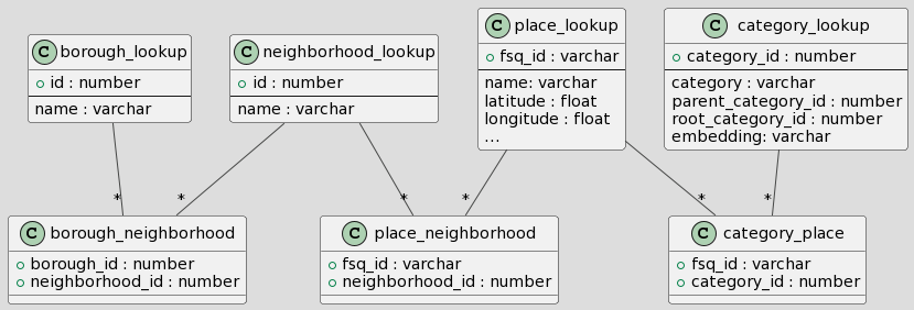
After all the data wrangling, we have transformed the original Foursquare view into the following relational tables:

With data wrangling out of the way, let’s move on to the fun stuff…

Implementations

The goal is to use Snowflake to compute cosine similarities between the embeddings of the user query (such as "Epic Night Out") and the embeddings of each Foursquare venue category. This will let us return the top suggested categories to the app, which can then look up venues with the suggested categories in the user-specified neighborhoods.

Initially, I planned to create a scalar User-Defined Function (UDF) for performing a semantic search via a quick table scan. But due to performance reasons (explained in the performance section), I abandoned this approach in favor of native SQL implementations. This section will cover the four implementations I explored: two Python scalar UDFs, one JavaScript scalar UDF, and native SQL. In the following sections, I will discuss their performances and scalability.

Implementation 1: Python UDF using an existing function

My first attempt was to wrap a readily available cosine similarity function within a Python UDF:

CREATE OR REPLACE FUNCTION cosine_similarity_score(x array, y array)
returns float 
language python 
runtime_version = '3.8'
packages = ('scikit-learn', 'numpy')
handler = 'cosine_similarity_py'
as 
$$
from sklearn.metrics.pairwise import cosine_similarity
import numpy as np

def cosine_similarity_py(x, y):
  x = np.array(x).reshape(1,-1)
  y = np.array(y).reshape(1,-1)
  cos_sim = cosine_similarity(x, y)
  return cos_sim 
$$;

The function above first transforms the 1D list into a 2D vector. It then uses scikit-learn's cosine similarity function to compute the similarity score between the two vectors.

Implementation 2: Python UDF with custom implementation

I noticed that OpenAI's embedding vectors normalize to length 1, which means that cosine similarity can be calculated using the dot product between the two vectors. So, I tried to write a Python UDF that doesn't require the scikit-learn package:

CREATE OR REPLACE FUNCTION cosine_similarity_score_2(x array, y array)
returns float 
language python 
runtime_version = '3.8'
packages = ('numpy')
handler = 'cosine_similarity_py'
as 
$$
import numpy as np

def cosine_similarity_py(x, y):
  x = np.array(x)
  y = np.array(y)
  return np.dot(x,y)
$$;

The function above transforms the 1D lists into NumPy arrays and computes the dot products of the two input arrays.

Implementation 3: JavaScript UDF with custom implementation

I also implemented a JavaScript UDF version, wondering how it would perform:

CREATE OR REPLACE FUNCTION cosine_similarity_score_js(x array, y array)
  RETURNS float
  LANGUAGE JAVASCRIPT
AS
$$
  var score = 0;
  for (var i = 0; i < X.length; i++) {
    score += X[i] * Y[i];
  }
  return score;
$$
;

Implementation 4: Native SQL

Finally, I decided to implement cosine similarity directly with SQL. Before writing the query, I flattened the JSON array category embedding values and stored them in the category_embed_value table:

CREATE OR REPLACE TRANSIENT TABLE category_embed_value AS 
WITH leaf_category AS (
    SELECT category_id 
    FROM category_lookup 
    EXCEPT 
    SELECT category_id 
    FROM category_lookup 
    WHERE category_id IN (SELECT DISTINCT parent_category_id FROM category_lookup)
)
SELECT 
    l.category_id  
    , n.index 
    , n.value 
FROM category_lookup l 
, table(flatten(input => parse_json(l.embedding))) n 
WHERE l.category_id IN (SELECT category_id FROM leaf_category)
ORDER BY l.category_id, n.index;

Then I computed cosine similarities between a test input embedding vector vs. embeddings of all categories with the following SQL:

WITH base_search AS (
-- Karaoke Bar 
SELECT embedding FROM category_lookup where category_id = 13015
)
, search_emb AS (
SELECT 
    n.index
    , n.value 
from base_search l 
, table(flatten(input => parse_json(l.embedding))) n 
ORDER BY n.index
)
, search_emb_sqr AS (
SELECT index, value 
FROM search_emb r 
)
SELECT 
    v.category_id 
    , SUM(s.value * v.value) / SQRT(SUM(s.value * s.value) * SUM(v.value * v.value)) cosine_similarity 
FROM search_emb_sqr s 
INNER JOIN category_embed_value v ON s.index = v.index 
GROUP BY v.category_id
ORDER BY cosine_similarity DESC 
LIMIT 5;

Performance evaluation

I evaluated the performance of each implementation using an X-Small warehouse. The test was to find categories (out of 853 Foursquare venue categories) that most closely match the embedding of a test category. I tested each implementation twice (and made sure to wait for the warehouse to spin down before moving on to a different implementation).

I tested the first three implementations using the following query:

WITH user_embedding AS (
-- Karaoke Bar 
SELECT embedding FROM category_lookup where category_id = 13015
)
SELECT FUNCTION_NAME(parse_json(d.embedding), parse_json(c.embedding)) cosine_similarity, c.category_id  
FROM user_embedding d, 
category_lookup c
ORDER BY cosine_similarity DESC 
LIMIT 5;

I verified the native SQL implementation using the query mentioned above.

Here are the test results:

• Python UDF 1: 9 seconds for the initial query, 5 seconds on the subsequent run
• Python UDF2: 7.5 seconds initially, 4 seconds on the subsequent run
• Javascript UDF: 11 seconds, 11 seconds on the subsequent run
• Native SQL: 1.2 seconds, 564 milliseconds on the subsequent run (due to 24-hour query caching)

I was surprised by the significant performance difference between the UDF and SQL implementation (UDFs didn’t seem to benefit from Snowflake's native query caching). I expected some language overhead for the UDFs, but not an 8x difference. Given the performance numbers, I proceeded with the native SQL implementation for the app.

Scalability evaluation

Semantically searching across 853 categories was exciting, but how scalable is it? To test scalability, I ran the native SQL solution against dummy datasets containing 10K, 100K, and 1M documents.

I created this SQL dummy table to hold embedding values for 10K, 100K, and 1M documents:

CREATE OR REPLACE TRANSIENT TABLE test_embed_value_10K AS 
WITH dummy_data AS (
  SELECT
    SEQ4() AS id,
    UNIFORM(1, 1000, SEQ4()) AS category_id,
    UNIFORM(1, 1536, SEQ4()) AS index,
    UNIFORM(0, 1, SEQ4()) AS value
  FROM
   -- Each embedding vector contains 1536 numbers 
    TABLE(GENERATOR(ROWCOUNT => 1536 * 10000))
)

SELECT *
FROM dummy_data
ORDER BY category_id, index;

I adjusted the row count in the TABLE(GENERATOR(ROWCOUNT => ... clause and the table name to create tables for 100K and 1M documents.

I used the same query (but swapped out category_embed_value with the test table name) to evaluate the scalability of the SQL implementation. Here are the results on an X-Small warehouse:

• 10K: 1.4 seconds
• 100K: 4.6 seconds
• 1M: 36 seconds

One of Snowflake’s benefits is its scalability. Performances can be further improved by using a larger warehouse.

Wrapping up

From this exploration, we show that Snowflake can not only power a semantic search application but also performs well when searching through up to 10K documents. Compared to keyword-based search, semantic search provides a better user experience by letting users search with intent or keywords. Ambiguous searches yield a diverse array of suggestions, while targeted searches continue to return targeted results. For example, "epic night out" returns “night club”, “beer bar”, and “escape room”. "Dim sum" returns "dim sum restaurants".

With more time, I’d have refined the project by creating a Snowflake external function to call OpenAI's embedding API, allowing me to embed new documents directly within Snowflake. Also, I’d set up a stored procedure and a scheduled task to automatically refresh the cached Foursquare data.

If you're already using Snowflake, conducting reasonably-sized semantic searches within it is possible, rather than setting up additional ETL jobs to push your data to a vector database. A capacity of 10K documents is more than enough for many applications. For example, you can search across embeddings of a book's paragraphs or chat sessions (stored in logically segregated tables for each natural grouping). Snowflake can still be a viable solution for larger document corpora depending on your use case and the compute resources you're willing to invest.

Stay tuned for Part 2, where I will discuss implementing the rest of the application with Snowflake and Streamlit. I hope you enjoyed my second article (my first article was about building GPT Lab with Streamlit). Connect with me on Twitter or Linkedin. I'd love to hear from you.