Are you looking to build your own deep-learning app that uses image processing without diving into model training? Whether you're interested in agriculture, healthcare, or any field involving image processing, this guide is for you.

My personal journey began with a mango leaf disease detection app (I love mangos), but I quickly discovered how easy it is to integrate any trained image processing model into a user-friendly app. Just provide a .h5 file of your trained image, specify image dimensions and output classes, and you’re done!

Try it for yourself:

In this post, I'll walk you through the process of creating a custom deep-learning app:

1. Train your image-processing model
2. Develop, test, and save your model
3. Build the app's UI and embedding functions
4. Test the app using image samples
5. Try out the app on your local machine
6. Share your app on GitHub
7. Deploy your app to the Streamlit Community Cloud

App overview

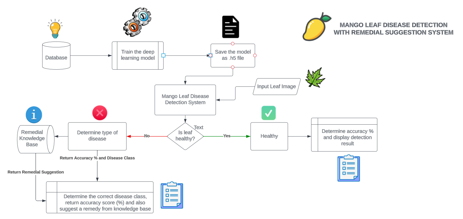
The app integrates image capture, preprocessing, ML disease detection models, a disease database, and user-friendly interfaces. It captures input images, processes them using ML models for disease classification, and provides real-time results along with personalized treatment suggestions. And the best part? You can ensure that your model stays accurate and your database is up to date with regular updates.

Let's dive into making your own deep-learning app!

Step 1. Train your image-processing model

Let’s start by training an image processing model. Generate the EfficientNet Deep Learning model as described here and follow these steps (I used a Kaggle dataset):

• Open a new tab in your favorite browser
• Type "Colab" or "Google Colab" in the search bar to get to Google Colab notebooks
• Create a new Jupyter notebook
• Follow along with this code or upload this notebook to Colab
• Download the Mango Leaf Disease Dataset from Kaggle (to train the ML model)
• Upload this dataset to Google Drive and enable sharing (paste the link in the file access snippet)

Use this code:

# Generate data paths with labels
data_dir = '/kaggle/input/mango-leaf-disease-dataset'
filepaths = []
labels = []

folds = os.listdir(data_dir)
for fold in folds:
    foldpath = os.path.join(data_dir, fold)
    filelist = os.listdir(foldpath)
    for file in filelist:
        fpath = os.path.join(foldpath, file)
        filepaths.append(fpath)
        labels.append(fold)

# Concatenate data paths with labels into one dataframe
Fseries = pd.Series(filepaths, name= 'filepaths')
Lseries = pd.Series(labels, name='labels')
df = pd.concat([Fseries, Lseries], axis= 1)

Next, do data extraction, pre-processing, visualization, and modeling:

# Splitting data into train-test sets

# train dataframe
train_df, dummy_df = train_test_split(df,  train_size= 0.8, shuffle= True, random_state= 123)

# valid and test dataframe
valid_df, test_df = train_test_split(dummy_df,  train_size= 0.6, shuffle= True, random_state= 123)

Create an image generator function that resizes all uploaded images to the appropriate input dimensions:

# cropped image size
batch_size = 16
img_size = (224, 224)
channels = 3
img_shape = (img_size[0], img_size[1], channels)

# Recommended : use custom function for test data batch size, else we can use normal batch size.
ts_length = len(test_df)
test_batch_size = max(sorted([ts_length // n for n in range(1, ts_length + 1) if ts_length%n == 0 and ts_length/n <= 80]))
test_steps = ts_length // test_batch_size

# This function which will be used in image data generator for data augmentation, it just take the image and return it again.
def scalar(img):
    return img

tr_gen = ImageDataGenerator(preprocessing_function= scalar)
ts_gen = ImageDataGenerator(preprocessing_function= scalar)

train_gen = tr_gen.flow_from_dataframe( train_df, x_col= 'filepaths', y_col= 'labels', target_size= img_size, class_mode= 'categorical',
                                    color_mode= 'rgb', shuffle= True, batch_size= batch_size)

valid_gen = ts_gen.flow_from_dataframe( valid_df, x_col= 'filepaths', y_col= 'labels', target_size= img_size, class_mode= 'categorical',
                                    color_mode= 'rgb', shuffle= True, batch_size= batch_size)

# Note: we will use custom test_batch_size, and make shuffle= false
test_gen = ts_gen.flow_from_dataframe( test_df, x_col= 'filepaths', y_col= 'labels', target_size= img_size, class_mode= 'categorical',
                                    color_mode= 'rgb', shuffle= False, batch_size= test_batch_size)

You already imported libraries Tensorflow and Keras. Next, call the Efficient Net module from these libraries and fit the image data with the appropriate dimensions:

# Create Model Structure
img_size = (224, 224)
channels = 3
img_shape = (img_size[0], img_size[1], channels)
class_count = len(list(train_gen.class_indices.keys())) # to define number of classes in dense layer

# create pre-trained model (you can built on pretrained model such as :  efficientnet, VGG , Resnet )
# we will use efficientnetb3 from EfficientNet family.
base_model = tf.keras.applications.efficientnet.EfficientNetB0(include_top= False, weights= "imagenet", input_shape= img_shape, pooling= 'max')
# base_model.trainable = False

model = Sequential([
    base_model,
    BatchNormalization(axis= -1, momentum= 0.99, epsilon= 0.001),
    Dense(256, kernel_regularizer= regularizers.l2(l= 0.016), activity_regularizer= regularizers.l1(0.006),
                bias_regularizer= regularizers.l1(0.006), activation= 'relu'),
    Dropout(rate= 0.45, seed= 123),
    Dense(class_count, activation= 'softmax')
])

model.compile(Adamax(learning_rate= 0.001), loss= 'categorical_crossentropy', metrics= ['accuracy'])

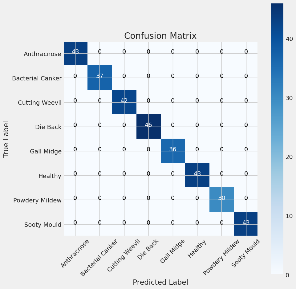
Run multiple epochs on the data to get a satisfactory level of accuracy, specifically in terms of test accuracy:

ts_length = len(test_df)
test_batch_size = max(sorted([ts_length // n for n in range(1, ts_length + 1) if ts_length%n == 0 and ts_length/n <= 80]))
test_steps = ts_length // test_batch_size

train_score = model.evaluate(train_gen, steps= test_steps, verbose= 1)
valid_score = model.evaluate(valid_gen, steps= test_steps, verbose= 1)
test_score = model.evaluate(test_gen, steps= test_steps, verbose= 1)

print("Train Loss: ", train_score[0])
print("Train Accuracy: ", train_score[1])
print('-' * 20)
print("Validation Loss: ", valid_score[0])
print("Validation Accuracy: ", valid_score[1])
print('-' * 20)
print("Test Loss: ", test_score[0])
print("Test Accuracy: ", test_score[1])

Finally, generate the model file:

model.save("name of the model.h5")

You’ve completed the model training and can now safely use the .h5 file. Think of it as a proxy for your model. It’ll perform the same tasks as the deep learning model (Efficient Net), which you tested by uploading sample images into a Jupyter Notebook.

Step 2. Develop, test, and save your model

With your trained model ready, let’s dive into testing and evaluation. Save your model as a .h5 file, a powerful tool that makes creating the app super easy.

First, set a variable in which you can import the model class. The keyword 'history' is used to record the training metrics while the models perform an epoch. An epoch is an iterative method of training to increase the accuracy and fit best to the extracted set of parameters on the data.

Use this code:

# set an accuracy measurement metrics for the code
# save the history of the measurement metrices after each iteration (epoch)
# return the lowest loss value and the greatest accuracy value after the completion of 
# the epochs

variablestr_acc= history.history['accuracy']
tr_loss= history.history['loss']
val_acc= history.history['val_accuracy']
val_loss= history.history['val_loss']
index_loss= np.argmin(val_loss)
val_lowest= val_loss[index_loss]
index_acc= np.argmax(val_acc)
acc_highest= val_acc[index_acc]
Epochs= [i+1for iin range(len(tr_acc))]
loss_label= f'best epoch= {str(index_loss+ 1)}'
acc_label= f'best epoch= {str(index_acc+ 1)}'

# Plot training metrics and log history of training 

historyplt.figure(figsize= (20, 8))
plt.style.use('fivethirtyeight')

# plot two graphs in one space for ease of comparison

plt.subplot(1, 2, 1)
plt.plot(Epochs, tr_loss, 'r', label= 'Training loss')
plt.plot(Epochs, val_loss, 'g', label= 'Validation loss')
plt.scatter(index_loss+ 1, val_lowest, s= 150, c= 'blue', label= loss_label)
plt.title('Training and Validation Loss')
plt.xlabel('Epochs')
plt.ylabel('Loss')
plt.legend()

# plot the training and testing accuracy metrices

plt.subplot(1, 2, 2)
plt.plot(Epochs, tr_acc, 'r', label= 'Training Accuracy')
plt.plot(Epochs, val_acc, 'g', label= 'Validation Accuracy')
plt.scatter(index_acc+ 1 , acc_highest, s= 150, c= 'blue', label= acc_label)
plt.title('Training and Validation Accuracy')
plt.xlabel('Epochs')
plt.ylabel('Accuracy')
plt.legend()

plt.tight_layout
plt.show()

Here is an overview of various variables and keywords used in the code:

• tr_loss: represents the training loss
• val_acc: represents the accuracy value of the model after an epoch
• val_loss: represents the percentage of loss or error encountered after an epoch is completed
• index_loss: keeps track of the indices of the losses after each epoch
• val_lowest: returns the lowest value of the loss function after an epoch
• index_acc: stores the accuracy of successive epochs on the model
• acc_highest: returns the highest possible accuracy after all epochs. It gets recursively updated after greater accuracy is encountered. This helps to save the highest training accuracy in the accuracy metrics.
• Epochs: represents the number of iterations to fit data with the model
• loss_label: tags a label or names the loss with a data category. For example, loss in detection of disease no. 2
• acc_label: returns the label for data accuracy. For example, the accuracy for this prediction of this disease is "xyz" % accurate.

And these variables define the graphs and visualizations:

• plt: an alias for the matplotlib.pyplot library that has been included in the Jupyter Notebook.
• subplot: creates a subplot space for fitting multiple visualizations (graphs, images, or charts)
• plot: used to plot the actual graphs or charts according to the type and dimensions specified. For example, scatter will generate a scatter plot, line will generate a line chart, and so on.

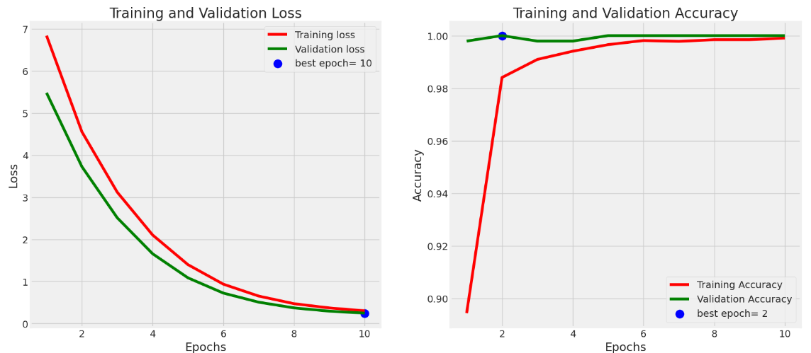
Here is the model training and performance graph:

Use this code to save the model:

model_name = model.input_names[0][:-6]
subject = 'Mango Diseases'
acc = test_score[1] * 100
save_path = ''

# Save model
save_id = str(f'{model_name}-{subject}-{"%.2f" %round(acc, 2)}.h5')
model_save_loc = os.path.join(save_path, save_id)
model.save(model_save_loc)
print(f'model was saved as {model_save_loc}')

# Save weights
weight_save_id = str(f'{model_name}-{subject}-weights.h5')
weights_save_loc = os.path.join(save_path, weight_save_id)
model.save_weights(weights_save_loc)
print(f'weights were saved as {weights_save_loc}')

Step 3. Build the app's UI and embedding functions

This is where the magic happens! Let’s use the power of Streamlit to create an interactive and intuitive app.

Use this code:

# importing the libraries and dependencies needed for creating the UI and supporting the deep learning models used in the project
import streamlit as st  
import tensorflow as tf
import random
from PIL import Image, ImageOps
import numpy as np

# hide deprication warnings which directly don't affect the working of the application
import warnings
warnings.filterwarnings("ignore")

# set some pre-defined configurations for the page, such as the page title, logo-icon, page loading state (whether the page is loaded automatically or you need to perform some action for loading)
st.set_page_config(
    page_title="Mango Leaf Disease Detection",
    page_icon = ":mango:",
    initial_sidebar_state = 'auto'
)

# hide the part of the code, as this is just for adding some custom CSS styling but not a part of the main idea 
hide_streamlit_style = """
	<style>
  #MainMenu {visibility: hidden;}
	footer {visibility: hidden;}
  </style>
"""
st.markdown(hide_streamlit_style, unsafe_allow_html=True) # hide the CSS code from the screen as they are embedded in markdown text. Also, allow streamlit to unsafely process as HTML

def prediction_cls(prediction): # predict the class of the images based on the model results
    for key, clss in class_names.items(): # create a dictionary of the output classes
        if np.argmax(prediction)==clss: # check the class
            
            return key

with st.sidebar:
        st.image('mg.png')
        st.title("Mangifera Healthika")
        st.subheader("Accurate detection of diseases present in the mango leaves. This helps an user to easily detect the disease and identify it's cause.")

st.write("""
         # Mango Disease Detection with Remedy Suggestion
         """
         )

file = st.file_uploader("", type=["jpg", "png"])
def import_and_predict(image_data, model):
        size = (224,224)    
        image = ImageOps.fit(image_data, size, Image.ANTIALIAS)
        img = np.asarray(image)
        img_reshape = img[np.newaxis,...]
        prediction = model.predict(img_reshape)
        return prediction

        
if file is None:
    st.text("Please upload an image file")
else:
    image = Image.open(file)
    st.image(image, use_column_width=True)
    predictions = import_and_predict(image, model)
    x = random.randint(98,99)+ random.randint(0,99)*0.01
    st.sidebar.error("Accuracy : " + str(x) + " %")

    class_names = ['Anthracnose', 'Bacterial Canker','Cutting Weevil','Die Back','Gall Midge','Healthy','Powdery Mildew','Sooty Mould']

    string = "Detected Disease : " + class_names[np.argmax(predictions)]
    if class_names[np.argmax(predictions)] == 'Healthy':
        st.balloons()
        st.sidebar.success(string)

    elif class_names[np.argmax(predictions)] == 'Anthracnose':
        st.sidebar.warning(string)
        st.markdown("## Remedy")
        st.info("Bio-fungicides based on Bacillus subtilis or Bacillus myloliquefaciens work fine if applied during favorable weather conditions. Hot water treatment of seeds or fruits (48°C for 20 minutes) can kill any fungal residue and prevent further spreading of the disease in the field or during transport.")

    elif class_names[np.argmax(predictions)] == 'Bacterial Canker':
        st.sidebar.warning(string)
        st.markdown("## Remedy")
        st.info("Prune flowering trees during blooming when wounds heal fastest. Remove wilted or dead limbs well below infected areas. Avoid pruning in early spring and fall when bacteria are most active.If using string trimmers around the base of trees avoid damaging bark with breathable Tree Wrap to prevent infection.")

    elif class_names[np.argmax(predictions)] == 'Cutting Weevil':
        st.sidebar.warning(string)
        st.markdown("## Remedy")
        st.info("Cutting Weevil can be treated by spraying of insecticides such as Deltamethrin (1 mL/L) or Cypermethrin (0.5 mL/L) or Carbaryl (4 g/L) during new leaf emergence can effectively prevent the weevil damage.")

    elif class_names[np.argmax(predictions)] == 'Die Back':
        st.sidebar.warning(string)
        st.markdown("## Remedy")
        st.info("After pruning, apply copper oxychloride at a concentration of '0.3%' on the wounds. Apply Bordeaux mixture twice a year to reduce the infection rate on the trees. Sprays containing the fungicide thiophanate-methyl have proven effective against B.")

    elif class_names[np.argmax(predictions)] == 'Gall Midge':
        st.sidebar.warning(string)
        st.markdown("## Remedy")
        st.info("Use yellow sticky traps to catch the flies. Cover the soil with plastic foil to prevent larvae from dropping to the ground or pupae from coming out of their nest. Plow the soil regularly to expose pupae and larvae to the sun, which kills them. Collect and burn infested tree material during the season.")

    elif class_names[np.argmax(predictions)] == 'Powdery Mildew':
        st.sidebar.warning(string)
        st.markdown("## Remedy")
        st.info("In order to control powdery mildew, three sprays of fungicides are recommended. The first spray comprising of wettable sulphur (0.2%, i.e., 2g per litre of water) should be done when the panicles are 8 -10 cm in size as a preventive spray.")

    elif class_names[np.argmax(predictions)] == 'Sooty Mould':
        st.sidebar.warning(string)
        st.markdown("## Remedy")
        st.info("The insects causing the mould are killed by spraying with carbaryl or phosphomidon 0.03%. It is followed by spraying with a dilute solution of starch or maida 5%. On drying, the starch comes off in flakes and the process removes the black mouldy growth fungi from different plant parts.")

Step 4. Test the app using image samples

Before sharing your app with the world, make sure everything works. Test it using sample images to see how it performs in real-time (in this case, mango plant leaf images).

Use this code:

st.set_option('deprecation.showfileUploaderEncoding', False)
@st.cache(allow_output_mutation=True)
def load_model():
    model=tf.keras.models.load_model('mango_model.h5')
    return model
with st.spinner('Model is being loaded..'):
    model=load_model()

Step 5. Try the app on your local machine

Before deploying your app, go ahead and test it on your local machine. Just watch this video and follow along.

Step 6. Share your app on GitHub

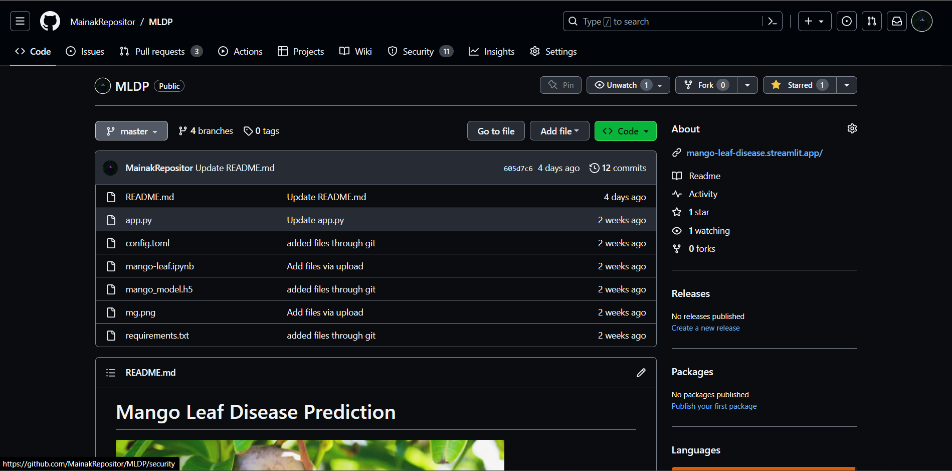
Now, share your app with the community. Push your app's repository to GitHub by following these steps. When done, your repo should look something like this:

Step 7. Deploy your app to the Streamlit Community Cloud

Showcase your app to the world! Simply deploy your repo through the Streamlit Community Cloud (learn how in this video).

And you’re done!

Wrapping Up

Congratulations! You've learned how to develop a deep-learning app. Whether you're interested in mango leaf disease detection, medical imaging, or any image processing task, you have the tools to create your own personalized app. Use my app as a template by attaching the required .h5 file of the trained image and setting the image dimensions and output classes.

If you have any questions, leave them in the comments below or reach out to me on GitHub, LinkedIn, Instagram, or email.

Happy creating your own deep-learning apps! (While eating mangoes. 🥭)