Hey, community! 👋

My name is Kanak, and I’m a Cloud Quality and Reliability Intern at Zscaler. The world of AI never ceases to amaze me. I enjoy learning about new technologies and tools that can help me solve complex problems and make data-driven decisions. Last year, during a hackathon, I built Deforgify—an app that detects fake images. It received a $1,000 grant from the 1517 community!

In this post, I’ll walk you through the seven steps of making it:

1. Collecting the dataset
2. Preprocessing images
3. Splitting the dataset
4. Designing the model architecture
5. Training the model
6. Evaluating the model
7. Building the UI

Want to jump right in? Here's the app and the repo code.

But first, I’d love to share with you…

Why did I decide to make it?

Generative Adversarial Networks (GANs) have been successful in deep learning, particularly in generating high-quality images that are indistinguishable from originals. However, GANs can also generate fake faces that deceive both humans and machine learning (ML) classifiers. There are many tutorials on YouTube that show how to use software such as Adobe Photoshop to create synthetic photographs—to be easily shared on social media and used for defamation, impersonation, and factual distortion.

I created Deforgify to leverage the power of deep learning in distinguishing real images from fake ones. This means that if someone were to Photoshop your face onto someone else's body, Deforgify would evaluate it and tag it as fake in a fraction of a second!

Now, let’s build the app step-by-step.

Step 1. Collecting the dataset

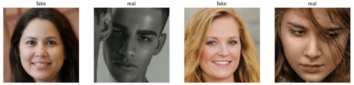
Download the dataset of real and fake faces from Kaggle. It has 1,288 faces—589 real and 700 fake ones. The fake faces were generated using StyleGAN2, which presents a harder challenge to classify them correctly (even for the human eye):

Step 2. Preprocessing images

To build an effective neural network model, you must carefully consider the input data format. The most common parameters for image data input are the number of images, the image's height and width, and the number of channels. Typically, there are three channels of data corresponding to the colors Red, Green, and Blue (RGB), and the pixel levels are usually [0,255].

Make a function that accepts an image path, reads it from the disk, applies all the pre-processing steps, and returns it. Use the OpenCV library for reading and resizing images, and NumPy for normalization:

def read_and_preprocess(img_path):
		# reading the image
    img = cv2.imread(img_path, cv2.IMREAD_COLOR)
		# resizing it to 128*128 to ensure that the images have the same size and aspect ratio. (IMAGE_SIZE is a global variable)
    img = cv2.resize(img, (IMAGE_SIZE, IMAGE_SIZE))
		# convert its datatype so that it could be normalized
    img = np.array(img, dtype='float32') 
		# normalization (now every pixel is in the range of 0 and 1)
    img = img/255 
    return img

Step 3: Splitting the dataset

Splitting the dataset is an important but often overlooked step in the ML process. It helps prevent overfitting, which occurs when a model learns the noise in the training data instead of the underlying pattern. This can result in a model that performs well on the training data but poorly on the testing data. By splitting the dataset, you can evaluate the model's performance on unseen data and avoid overfitting.

Another reason for splitting is to ensure that the model is generalizable. A model that is trained on a specific dataset may not perform well on new, unseen data. By splitting the dataset into training and testing sets, you can train the model on one set of data and evaluate its performance on another set, ensuring that it can handle new data.

I did 80% training, 10% testing, and 10% validation data split in such a way that:

1. The samples were shuffled
2. The ratio of each class was maintained (stratify)
3. Every time the data was split, it generated the same samples (random-state)

Stratifying while splitting data ensures that the distribution of the target classes in the training and testing sets is representative of the overall population.

For example, let's say you have a dataset of 1,000 individuals, 700 of which are men and 300 are women. You want to build a model to predict whether an individual has a certain medical condition or not. If you randomly split the data into a 70% training and 30% testing split without stratifying, it's possible that the testing set could have significantly fewer women than the training set. This could result in the model being biased towards men, leading to poor performance when predicting the medical condition in women.

On the other hand, if you stratify the data based on the gender variable, you ensure that both the training and testing sets have the same proportion of men and women. For instance, you could stratify the data so that the training set has 490 men and 210 women, and the testing set has 210 men and 90 women. This ensures that your model is trained on a representative sample of both genders, and it should therefore be more accurate when predicting the medical condition for both men and women.

Using the random_state parameter ensures that the same data is obtained each time you split the dataset. This lets you replicate your analysis and results, which is crucial for reproducibility. Without setting a random seed, each split of the data may be different, leading to inconsistent results.

Setting a random state is also important when you're sharing your work with others or comparing your results. If different individuals are using different random seeds, they may end up with different results even if they use the same code and dataset.

Step 4. Designing the model architecture

It’s possible that a model architecture, which has worked well on one problem statement, could work well on other problem statements as well. This is because the underlying ML concepts and techniques are often applicable across different domains and problem statements.

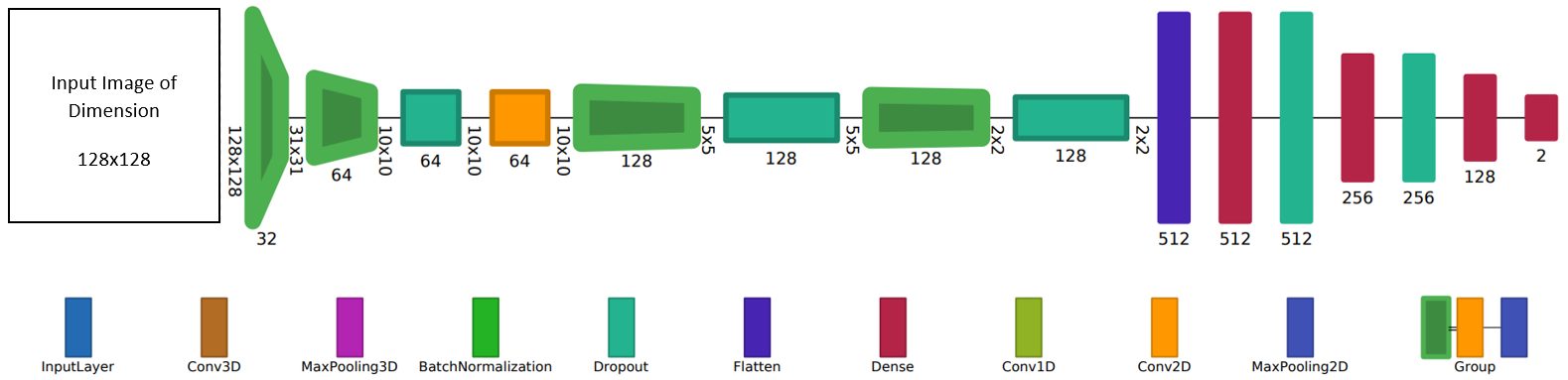
After reading numerous research papers and experimenting, I have designed my own model architecture that I use across all my projects (with minor tweaks):

• It consists of a sequential model with five convolutional layers and four dense layers.
• The first convolutional layer has 32 filters and a kernel size of 2x2.
• At each subsequent convolutional layer, the number of filters is doubled, and the kernel size is incremented by one.
• To reduce overfitting and computational costs, max-pooling layers are introduced after each convolutional layer.
• The output from the convolutional layer is flattened and passed to the dense layers.
• The first dense layer has 512 neurons, and the number of neurons is halved in the next two dense layers.
• Dropout layers are introduced throughout the model to randomly ignore some neurons and reduce overfitting.
• ReLU activation is used in all layers except for the output layer, which has two neurons (one for each class) and softmax activation.

Step 5. Training the model

Compiling an ML model involves configuring its settings for training. The three key settings to consider are:

1. The loss function: It measures the difference between the predicted output and the actual output of the model. The choice of loss function depends on the type of problem being solved. Since you're performing classification and your training labels are represented in categorical format (0,1), sparse_categorical_crossentropy is the logical choice.
2. The optimizer: It updates the weights of the model during training to minimize the loss function. Some popular optimizer algorithms include stochastic gradient descent, Adam, and RMSprop. The choice of optimizer depends on the complexity of the problem and the size of the dataset. The Adam optimizer works well in most cases, so "when in doubt, go with Adam!"
3. The evaluation: It measures the performance of the model during training and validation. Since your dataset is pretty balanced, there is no harm in going with accuracy.

Hyperparameters such as the learning rate, batch size, number of epochs, and regularization parameters can also be adjusted during model compilation.

The two optional steps that help improve the model’s performance and save training time are:

Early stopping: It prevents overfitting and reduces training time by monitoring the performance of the model on a validation set during training. It stops the training process once the model's performance on the validation set starts to decrease, indicating that it’s reached its optimal performance. Early stopping can save time and computational resources and prevent the model from overfitting to the training data. You’re going to configure early stopping to monitor minimum validation loss with the patience of 10, which means that if the validation loss doesn’t reduce for 10 continuous epochs, the model training will be stopped:

from tensorflow.keras.callbacks import EarlyStopping
earlystopping = EarlyStopping(monitor='val_loss', mode='min', verbose=1, patience=10)

Checkpointer: It saves the model's weights at specific intervals during training. This enables the model to resume training from where it stopped in the event that the process is halted due to an error or other issue. The checkpointer stores the weights in a file that can be loaded later to resume training. Checkpointing is particularly beneficial for large models that take a long time to train, as it allows the training process to continue without starting over. To set the checkpointer to save only the best model (i.e., one with the least validation loss), follow these steps:

from tensorflow.keras.callbacks import ModelCheckpoint
checkpointer = ModelCheckpoint(filepath="fakevsreal_weights.h5", verbose=1, save_best_only=True)

You’re now ready to train your model! Remember to pass in all the parameters that you have configured:

history = model.fit(X_train, y_train, epochs=100, validation_data=(X_val, y_val), batch_size=32, shuffle=True, callbacks=[earlystopping, checkpointer])

Step 6. Evaluating the model

Evaluating the performance of an ML model is crucial to assess its ability to generalize to new, unseen data. To reload it, use the load_model() function from the Keras library.

model = tf.keras.models.load_model('fakevsreal_weights.h5')

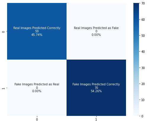
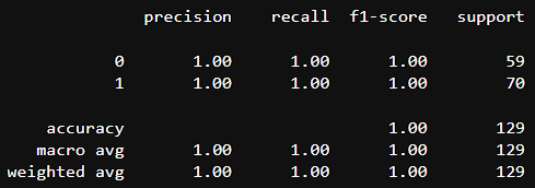
Make predictions on the testing data, evaluate its performance, and compute its accuracy, precision, recall, and F1-score using the confusion matrix:

Here is the complete classification report:

Step 7. Building the UI

The model's performance evaluation alone may not be sufficient to showcase its capability. End users might not have the necessary skills or time to write code and use the trained model. One solution is to build a user interface (UI) that allows users to interact with the model. However, this requires a different skillset that many users may not possess.

This is where Streamlit comes in! 🎈

With just 12 lines of code, you can create an interactive Streamlit app using Streamlit (this will showcase your skills and make your models accessible to a wider audience):

import streamlit as st
# util is a custom file that includes steps to read the model and run predictions on an image
import util

st.image('Header.gif', use_column_width=True)
st.write("Upload a Picture to see if it is a fake or real face.")
file_uploaded = st.file_uploader("Choose the Image File", type=["jpg", "png", "jpeg"])
if file_uploaded is not None:
    res = util.classify_image(file_uploaded)
    c1, buff, c2 = st.columns([2, 0.5, 2])
    c1.image(file_uploaded, use_column_width=True)
    c2.subheader("Classification Result")
    c2.write("The image is classified as **{}**.".format(res['label'].title()))

Here is the result:

But that's not all!

Deploying an ML app on the cloud can be a daunting task, even for experienced data scientists and developers. Fortunately, Streamlit makes it easy to deploy apps to their Streamlit Community Cloud platform with just a few clicks, without any complex configurations or infrastructure setup. To get started, create an account, obtain your app's code, and follow these steps.

Wrapping up

Thank you for reading my post! You learned how to make an image classifier that can distinguish between real and fake images, built a UI to showcase your model's capability to the world using Streamlit, and deploy it on the Streamlit Community Cloud.

If you have any questions, please post them in the comments below or contact me on Twitter, LinkedIn, or GitHub.

Happy Streamlit-ing! 🎈